Time series data and predictive maintenance

Contents:

• Time series data as a connector between building-blocks
• The basic rule: Do not estimate what you already know!
• The horseshoe model
• Phase 1: A classic finite element simulation of transient thermal stresses - but with open source software
• Phase 2: System identification by means of the Fast Fourier Transform
• Phase 2a: Investigating how a decomposition into components works
• Phase 3: Establishing a damage accumulation model
• Phase 4: Putting it all together into a 10 years lifetime simulation
• Phase 4a: Verifying that the identified model behaves like the original finite element model
• Phase 4b: A modification of thermal properties may extend the life of the horseshoe
• And this is only the beginning...

In a companion article, I have outlined the playground for time series data as a general means of communication between systems as well as between systems and humans. As stated here and here, people with an interest in predictive maintenance should take an interest in a special kind of time series: the damage parameter. Damage parameters may be chosen in lots of ways, but the basic idea stays the same: if the parameter value is way below 1, you should expect the component to have plenty of service life left. If the parameter rises above 1, you should expect the component to have failed or being very prone to failure.

Thus, a damage parameter is one out of many types of time series. The general ability to correctly predict a time series in the future is mandatory for the ability to predict when a spare part will fail. The glorious vision is the ability to do so for each individual instance of this spare part. A less ambitious goal - still with a big potential for profit - is the ability to estimate the average need for spare parts in the future.

Time series data as a connector between building-blocks

The idea of decomposing a complex engineering scenario into building-blocks has already been presented here. Such a graphical display embodies the basic rule to presented later: "Do not estimate what you already know". If you know the flow of effects leading to final damage, you should never consider an artificial intelligence procedure for doing the same job. It may utterly fail and you may never find out that it did.

I have found no iron-clad recipe concerning how to present a connection of concepts like that below:

Figure 1: A SimxonCARE view (the "network of causality") of the problem in Figure 2

I have chosen to put time series names into rectangular boxes and the processing of them into oval boxes. Keesman's monography referred to here applies the control theory idiom of putting processing into rectangular boxes and identify the time series through letters next to the arrows connecting the processing boxes. The reader is encouraged to view any presentation idiom with an open mind.

The basic rule: Do not estimate what you already know!

After this paragraph, 8 paragraphs follow which focus on a particular model problem. No additional general concepts are presented until the final paragraph. So, this is my last chance to highlight and your last chance to acknowledge that - although no particular references are made - the handling of the model problem follows this basic rule (also mentioned here):

The horseshoe model

This model problem has been presented previously:

Figure 2: A model thermomechanical problem

No actual mechanical device has a component like this. When subjected to heat transfer from a time-varying heat source up left, continuing trough the bend to a heat sink down left, mechanical stresses are generated at the fillet, leading to fatigue. Many actual mechanical components may suffer from fatigue due to heat transfer. Later on in this article, the model will be subjected to a time-varying heat load pattern typical for a wind turbine.

I have dubbed the model "the horseshoe" because the finite element realization of it features a soft bend (so that the stress maximum will be located at the fillet):

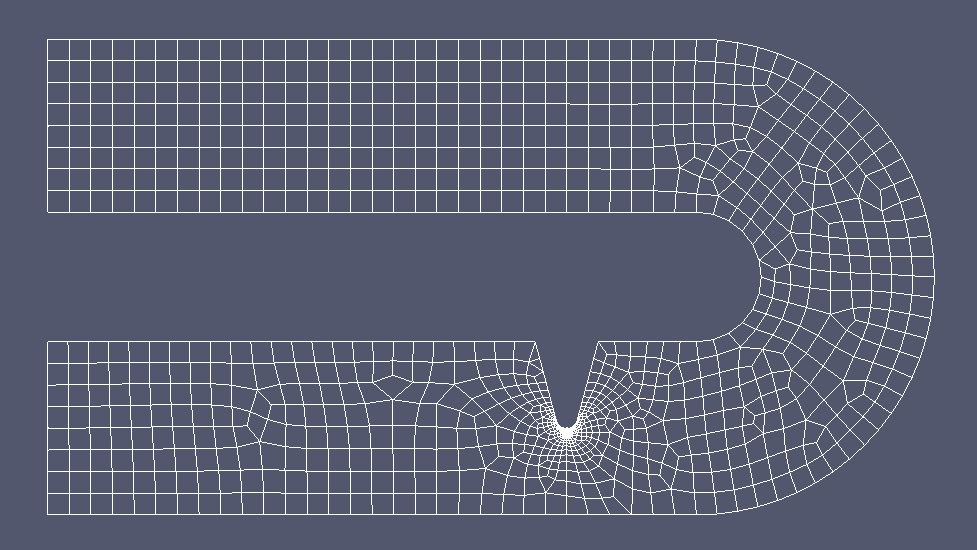
Figure 3: A "horseshoe" finite element model (2D parabolic elements) corresponding to Figure 2 above

Phase 1: A classic finite element simulation of transient thermal stresses - but with open source software

A typical thermal solution looks like this (as provided by the excellent French open source finite element program Code_Aster):

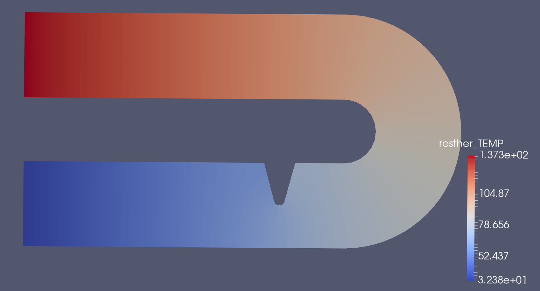
Figure 4: Horseshoe temperature distribution

, a stress solution looks like this:

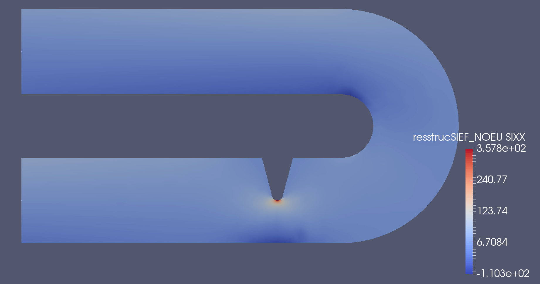
Figure 5: Horseshoe longitudinal stress distribution

and zooming in on the stress solution looks like this:

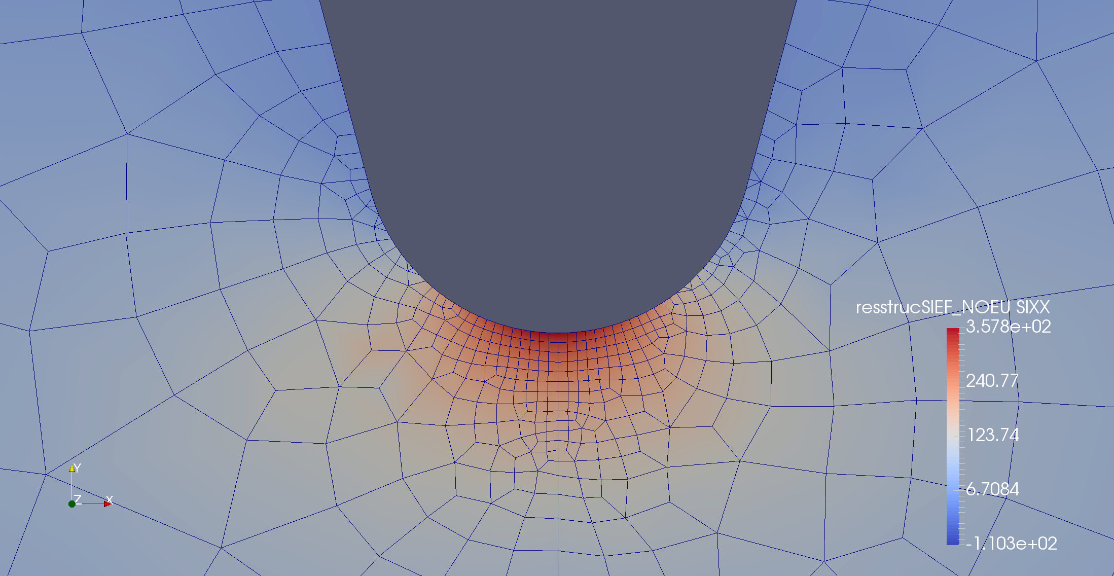
Figure 6: Zooming in on the horseshoe stress distribution

Phase 2: System identification by means of the Fast Fourier Transform

Figure 6 above strongly suggests that the longitudinal stress at the bottom of the fillet is very close to the maximum tensile stress occurring anywhere in the model. Assuming that to be true, the entire problem of determining maximum stress as a function of a time-varying heat load becomes linear. Applying a unit pulse (with the highest frequencies filtered out) and calculating the Fast Fourier Transform for a period much longer than the typical response time then lead to a transfer function which is quite reliable (Figures 7 and 10 below).

Do not underestimate the savings in computer resources due to this step. Repeating a transient thermomechanical analysis for a vast number of time steps is feasible for a small 2D model like this one. If the finite element step is a large-scale 3D simulation, the cost savings may be huge if you replace that by some small matrix operations!

Phase 2a: Investigating how a decomposition into components works

In the paragraphs to follow this one, the fillet stress is calculated directly from the heat load. In order to follow the idea (suggested in Figure 1 - the "network of causality" - above) of assuming

• the leftmost temperatures T1 and T2 to be functions of the heat load with respect to time, and then assuming
• the fillet stress to be a function of T1 and T2 with respect to time

, an alternative method of calculating the fillet stress as a function of the heat load is obtained. Figure 7 below compares the "direct approach" (FEM simulation without any FFT processing) with this indirect approach:

Figure 7: Two methods of calculating the fillet stress

The time axis of Figure 7 corresponds to two consecutive periods of the length used for FFT system identification (identification is always based on the last period). You see from the blue curve that it takes at least one period for things to stabilize. The yellow and the blue curve should only be compared for period number two.

Phase 3: Establishing a damage accumulation model

The introductory remarks of this article ends with stating that the discipline of predictive maintenance is tightly coupled with the concept of damage parameters. If you have a fillet stress as a function of time (obtained from the previous paragraphs), you can calculate the damage parameter as a function of time by applying

• an S-N curve,
• the rainflow counting procedure and
• Miner's Rule.

Figure 8 below shows the S-N curve assumed to the subsequent calculations. Steel has properties which look like this.

Figure 8: Fatigue stress as a function of the number of stress cycles

Phase 4: Putting it all together into a 10 years lifetime simulation

(see here for a 30 years calculation). Combining

• the computational cost savings from replacing a full-blown finite element simulation with an identified model,
• the three step recipe above of getting from stress as a function of time to damage as a function of time, and
• a "power as a function of time" curve which can be attributed to a real wind turbine

, you can generate a plot like Figure 9 below:

Figure 9: Power versus time displayed together with damage versus time

Phase 4a: Verifying that the identified model behaves like the original finite element model

Figure 10 below shows the same situation as that of the previous paragraph. The blue curve is the heat load, the yellow curve is the fillet stress calculated by a finite element simulation and the green curve results from the identification procedure described previously:

Figure 10: Power versus time displayed together with damage versus time

The FFT-based identification procedure draws on heat load data from the previous period length in order to calculate the next fillet stress value. As for Figure 7, it is therefore to be expected that the rightmost half of the plot provides a better match than the leftmost part (240 hours correspond to two identification periods).

Phase 4b: A modification of thermal properties may extend the life of the horseshoe

The calculation procedure leading to Figure 9 above may be modified so that lessons may be learned. For instance, Figure 10 shows that the fillet stress follows the heat load with a time delay so that fast load cycles lead to lower stress amplitudes than slow load cycles.

One way to decrease at least some of the load cycles is therefore to increase the time constant of the thermal problem. Just as an experiment, an additional heat capacity was therefore included next to the heat sink bottom left in Figure 2. Figure 9 is then modified to look like this:

Figure 11: Power versus time displayed together with damage versus time - now with reduced damage

Compared to Figure 9, the damage after 10 years of the same operation load history has decreased from 1.13 to 0.91 just from a modification of the thermal properties of the horseshoe.

And this is only the beginning...

This article documents how an automated procedure based entirely on software without marginal cost combines well-known and new elements into a procedure with an unusual predictive capability. Because Dijkstra's principle of separation of concerns has been strictly adhered to, everything is extremely adaptable and scalable. The horseshoe component was only meant for easy development work and a simple way of presenting fundamental properties of the SimxonCARE procedure.

Still, you ain't seen nothing yet. The proprietory procedure called CARE hasn't been drawn upon at all. CARE has the potential of handling nonlinear and otherwise complex issues which the realm of linearity considered in this article cannot handle.

And then there will be a transition from a prototype software environment like the one applied here to a professional software system in daily use. As all applications of SimxonCARE are expected to be highly customized, it is a good idea to deliberately stay on the software prototype level until all relevant decisions have been made and everything has been thoroughly tested.

Neither we nor our customers should at any time forget the abundance of time series prediction techniques described or referred to in this companion article.

We expect some or all of the following targets to be met in the future:

• The future need for spare parts can be predicted with a confidence unknown today.
• Simple embedded software can keep track of the remaining lifetime of each spare part instance. Spare parts may thus arrive in due time and at reduced freight rates.
• With the behavior of existing products analyzed and documented to an unprecedented extent, product development may lead to even better lifecycle properties.