CAE, statistics and robust design

Introduction

I have recently been rewired. For almost 60 years, I thought that 2+2 equaled 4. Now I have realized that a more appropriate way of putting it is this:

If a stochastic variable with an expected value of 2 is added to another stochastic variable with an expected value of 2, the sum will be a stochastic variable with an expected value of 4.

All those millions of floating point numbers which I have entered, programmed and passed on to colleagues were just stochastic variables with zero variance!

I have decided to catch up. A very bad metaphor: If you find yourself in my shoes, I hereby invite you to follow my footsteps...

A simple example: Designing a mass-produced rotor which will not create imbalance problems

I have worked with big industrial rotors for decades. They were all subjected to a final balancing operation before they were shipped. The center of gravity for several tons of steel only needs to be slightly displaced from the rotor axis in order to create problems. The same issue applies when balancing the wheels of a car.

If a rotor is to be mass-produced as part of a luxury item, final balancing is an unwanted complication. I have seen a proprietary study of such a problem. I cannot show you any pictures, but the general line of presentation goes like this:

The main parts are the rotor and a small number of rubber parts which provide centering and mechanical isolation.
The main dimensions of all parts should be regarded as stochastic variables.
Many of the main dimensions are otherwise free to choose. In particular, this goes for the rubber parts.
An interval of operational speed is given.
To have a critical speed (almost the same thing as an eigenfrequency) in that interval would be outright stupid.
A critical speed near the operational speed interval will, however, amplify the effect of any imbalance.
If important part dimensions are stochastic variables, imbalance is unavoidable.

What are then the optimal nominal dimensions for the rubber parts? The rubber parts should "tune away" resonance issues, and at the same time, their position and design should minimize the possibility of manufacturing operations leading to unnecessary eccentricity.

A general purpose, open source toolbox: OpenTURNS

According to this textbook, the French State was among the earliest adopters of combining Computer Aided Engineering (CAE) and statistics. Today, the company Phimeca offers their own proprietary software, PhimecaSoft. However, they also offer OpenTURNS in collaboration with Électricité de France (EDF). To the analysis engineer, OpenTURNS presents itself as a Python module.

I am so much of a newbie that I am unable to assess all OpenTURNS features. But - like many other high quality open source packages - OpenTURNS includes many usage examples which can be run at face value and subsequently experimented with.

I have experimented with this example:

from __future__ import print_function
import otsxutils
import openturns as ot
# Create the marginal distributions of the parameters
dist_E = ot.Beta(0.93, 3.2, 2.8e7, 4.8e7)
dist_F = ot.LogNormalMuSigma(30000, 9000, 15000).getDistribution()
dist_L = ot.Uniform(250, 260)
dist_I = ot.Beta(2.5, 4.0, 3.1e2, 4.5e2)
marginals = [dist_E, dist_F, dist_L, dist_I]
# Create the Copula
RS = ot.CorrelationMatrix(4)
RS[2, 3] = -0.2
# Evaluate the correlation matrix of the Normal copula from RS
R = ot.NormalCopula.GetCorrelationFromSpearmanCorrelation(RS)
# Create the Normal copula parametrized by R
copula = ot.NormalCopula(R)
# Create the joint probability distribution
distribution = ot.ComposedDistribution(marginals, copula)
distribution.setDescription(['E', 'F', 'L', 'I'])
# create the model
# model = ot.SymbolicFunction(['E', 'F', 'L', 'I'], ['F*L^3/(3*E*I)'])
fobj=otsxutils.OTSXFunction()
ifo=open("whatever.bash")
fobj.setScriptString(ifo.read().replace("runintempdir=1","runintempdir=0"))
ifo.close()
fobj.setMaxProcesses()
fobj.setXnames(["E","F","L","I"])
fobj.setYnames(["R"])
model=fobj.getFunction()
# create the event we want to estimate the probability
vect = ot.RandomVector(distribution)
G = ot.CompositeRandomVector(model, vect)
event = ot.Event(G, ot.Greater(), 30.0)
event.setName("deviation")
# Define a solver
optimAlgo = ot.Cobyla()
optimAlgo.setMaximumEvaluationNumber(1000)
optimAlgo.setMaximumAbsoluteError(1.0e-10)
optimAlgo.setMaximumRelativeError(1.0e-10)
optimAlgo.setMaximumResidualError(1.0e-10)
optimAlgo.setMaximumConstraintError(1.0e-10)
# Run FORM
algo = ot.FORM(optimAlgo, event, distribution.getMean())
algo.run()
result = algo.getResult()
# Probability
r1=result.getEventProbability()
print("r1 =",r1)
# Hasofer reliability index
r2=result.getHasoferReliabilityIndex()
print("r2 =",r2)
# Design point in the standard U* space
r3=result.getStandardSpaceDesignPoint()
print("r3 =",r3)
# Design point in the physical X space
r4=result.getPhysicalSpaceDesignPoint()
print("r4 =",r4)
# Importance factors
otsxutils.graphToSVG(result.drawImportanceFactors())
marginalSensitivity, otherSensitivity = result.drawHasoferReliabilityIndexSensitivity()
marginalSensitivity.setLegendPosition('bottom')
otsxutils.graphToSVG(marginalSensitivity)
marginalSensitivity, otherSensitivity = result.drawEventProbabilitySensitivity()
otsxutils.graphToSVG(marginalSensitivity)

If you compare the code sequence above with the original, you will see that I

have introduced a new (proprietary) Python module named "otsxutils".
have commented out the original definition of the computational model "model=ot.SymbolicFunction(['E', 'F', 'L', 'I'], ['F*L^3/(3*E*I)'])".
have introduced a new computational model defined by a bash script. This approach provides great flexibility in getting point output values from point input values. Derivatives, however, can only be calculated by means of difference schemes. There is no such thing as a free lunch.
have introduced a utility function which can create SVG files from OpenTURNS graphics output.
have discarded the last code lines. They require gradients and Hessians. OpenTURNS attempts to compute those numerically but apparently decides that it has failed.

The protocol for "whatever.bash" is simple: Input value assignments must appear literally in the script file (e.g., "E=30327533.3663"; the line will be edited by "otsxutils") - and output value(s) must be delivered in a "whatever.env" file with similarly styled floating point assignments (e.g., "R=29.9999713788").

I consider it off-topic to go into details with the contents of "whatever.bash". I will just point out that

any scriptable CAE package will do.
for the current problem, I noticed that "F*L^3/(3*E*I)" indicates the deflection of a cantilever beam,
so I applied pygmsh to create a beam model (with a fixed slenderness ratio of 50),
and applied Code_Aster to calculate the displacement "R" from the load "F".

otsxutils supports OpenTURNS multiprocessing. OpenTURNS attempts to multiprocess at least when calculating gradients and Hessians from point data without accompanying derivatives.

Read The Fine Textbook

If your first activity in this area is to read this textbook, you will get the historical perspective right and obtain a general overview of the possibilities. You will also be able to cross-reference the many strange method names of the OpenTURNS documentation with examples of how and why to apply them.

I have extracted these observations:

The general vehicle is called the isoprobabilistic transformation. Depending on the information you have to start with, this transformation may be performed more or less canonically and with more or less elegance. When you have done it, your reward is a rich palette of analysis approaches.
The author expresses a general dislike for in-between models (called metamodels, surrogate models, polynomial chaos, etc.). The same dislike is expressed in this article. An operational piece of advice seems to be: Use such models when you really need them, otherwise don't.

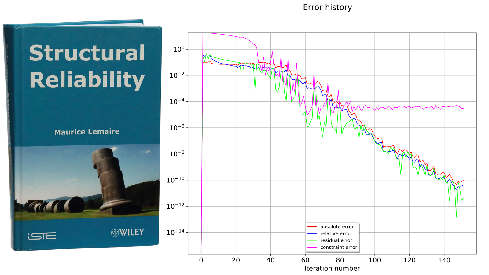
Some pictures

In order to verify that my latest calculation recipe (the one with a finite element beam calculation instead of a formula) ends up with the same result as the reference calculation, I created SVG files for every test run. They look like this:

A keen observer will notice that numeric values deviate slightly from the reference. I can live with that and suggest that you do the same.

I am not alone. You needn't be, either

I firmly believe that conglomerates of loosely coupled specialist companies may serve customers better than highly commercial top-down initiatives from the big CAE players. In that spirit,

Alter Ego Engineering (France)
Gmech Computing IVS (Denmark)
Kobe Innovation Engineering (Italy, not affiliated with Kobe Steel, Japan)
Simxon (Denmark)

are these days working on a joint marketing message. The two Danish companies have already fathered the SimxonCARE offering. The findings described above are part of our product development process.

We are definitely open for business. If you see yourself as either a paying customer or a contributor, do not hesitate to make contact.